The psyche clearly has structure. For example, patterns of behavior persist, resist perturbation, and occasionally reorganize in ways that look and feel discontinuous. A goal of psychologists over many years has been to provide a formal description of this structure in the hopes of developing better predictive and therapeutic tools.
A question we address here is whether that structure is accessible to mathematical description. Psychologists have thought so for a long time. William James described habit in 1890 as water cutting a channel in the landscape: repeated behavior deepens grooves that become progressively harder to escape. Jung's enantiodromia, the spontaneous reversal of a psychological state into its opposite, describes what a dynamical systems theorist would recognize as a transition between attractor basins. Kurt Lewin formalized the intuition in the 1930s with field theory, representing psychological forces as vectors in a topological space. The language of dynamics was present in psychology before the mathematics of chaos existed.
The first major mathematical treatment came with René Thom's catastrophe theory in the early 1970s, which modeled discontinuous transitions using the geometry of singularities. The framework was powerful, but its rapid adoption across the social sciences outpaced the available data, and the resulting skepticism slowed progress in mathematical approaches to psychology for years. Hermann Haken's synergetics provided a firmer foundation starting in 1975. A key contribution was the slaving principle: near critical transitions, complex systems with many degrees of freedom reduce to a few slow order parameters that dominate the macroscopic behavior while fast modes decay. Haken and Schiepek (2010) applied this framework directly to psychotherapy, arguing that therapeutic change can be understood as a self-organizing phase transition governed by low-dimensional order-parameter dynamics.
One of the most developed formal models to emerge from this program is Schiepek's five-variable system, coupling intensity of emotions, problem intensity, motivation to change, insight, and therapeutic success through nonlinear feedback (Schiepek et al., 2017; Schöller et al., 2018). Importantly, this is a system of five coupled nonlinear difference equations, not continuous-time differential equations. It produces dynamics consistent with the nonlinear psychotherapy literature: irregular fluctuations, critical instabilities preceding transitions, and phase-shift patterns that resemble what therapists report in practice. Separate empirical work by de Felice et al. (2022) found that good and poor outcomes differ in the degree of integration between cognitive and emotional-relational processing. Taken together, the evidence base for treating psychotherapy as a potentially nonlinear dynamical process is substantial and growing. What remains open is the correct reduced-order formulation.
So why do we want to reduce the dimensionality?
Schiepek's five-variable model is an important achievement, but five coupled state variables evolving in a five-dimensional space create a practical barrier: the dynamics cannot be directly visualized without projection. And projections from five to lower dimensions lose some of the coupling structure that generates the behavior. For researchers comfortable with high-dimensional analysis, this is workable. But for clinicians, clients, or anyone trying to recognize the shape of their own process of change, there is value in a native lower-dimensional representation that preserves the essential dynamical features while making them explicitly visible.
The Lorenz system lives in three dimensions, a level of dimensionality that humans work with every day. Its attractor has two wings that are immediately legible as two distinct behavioral states. Its control parameter produces a visible landscape of regimes: stability, intermittent switching, and chaos in the standard parameter range. The bifurcation diagram and Lyapunov exponent map are computable in real time. The geometry of the system is part of the argument. You do not need to be told that one wing is stable; you can watch a trajectory spiral into it and refuse to leave.
The formal justification for reducing from five variables to three rests on Haken's slaving principle. Near critical transitions, effective dimensionality drops. If the psyche near transition is governed by three dominant slow modes, the question becomes: what coupling topology do those three variables follow? The Lorenz topology is a strong candidate because it is not specific to any physical substrate. Closely related three-variable coupling structures arise in atmospheric convection (Lorenz, 1963) and in Haken's treatment of single-mode laser dynamics (Haken, 1975), and Lorenz-like dynamics have since appeared in other physical and biological settings. The coupling topology — which variables drive which, and through what nonlinear terms — is the invariant. The physical meaning of the variables changes with each domain, but the mathematics does not.
The EOC model is the hypothesis that this topology also governs psychological transition dynamics, with Engagement, Openness, and Consolidation as the three order parameters. What follows is the formal development of that hypothesis.
This work does not claim that the psyche is globally a Lorenz system. It claims that near major psychological transitions, a minimal set of order parameters may locally exhibit Lorenz-type dynamics. Specifically: the coupling topology of the Lorenz system (which variables drive which, and through what nonlinear terms) may capture the essential feedback structure that governs how engagement, openness, and consolidation interact during periods of acute reorganization.
The epistemological status is a plausible reduced-model conjecture consistent with the nonlinear psychotherapy literature. The model generates six testable predictions that distinguish it from linear models and from vague "therapy is nonlinear" formulations. The justification for the Lorenz topology rests on two pillars: the slaving principle from Haken's synergetics (which licenses low-dimensional reductions near critical transitions) and the Lorenz-Haken isomorphism (which demonstrates that this specific three-variable structure recurs across physical domains).
The formal mathematical framework is the EOC system presented here in brief; the fully developed framework is in Johnson, S.E. (2026). The companion interactive visualization implements the full system with real-time parameter control.
All variables are defined as signed deviations from a person's habitual baseline state. This formulation resolves a formal requirement of the Lorenz system: two of its three variables must be able to take negative values. By measuring deviation from baseline rather than absolute level, negative values acquire natural meaning (withdrawal rather than approach, rigidity rather than plasticity, pattern dissolution rather than pattern formation).
The EOC system consists of three coupled ordinary differential equations. With the identification $E = x$, $O = y$, $C = z$, this system is mathematically identical to Lorenz (1963). The mathematical results associated with the Lorenz system therefore apply to the EOC system without modification.
Engagement relaxes toward the current level of openness with rate constant $\sigma$. This is the least empirically grounded equation. It is retained as a closure assumption for parsimony and exact Lorenz equivalence, not because current data uniquely imply this specific coupling. The system is bidirectionally coupled: E influences O through Equation 2, and O influences E through Equation 1. Causality is circular and simultaneous, not unidirectional.
A natural question: how does the therapeutic process begin in a defended client whose baseline has both O and E near zero? The answer lies in the control parameter $\rho$. When $\rho > 1$, the origin becomes an unstable saddle point. Any infinitesimal perturbation is amplified. The system does not need a large push to leave baseline. It needs a $\rho$ large enough that baseline itself becomes unstable.
Three components, each with independent justification. The product $E(\rho - C)$ encodes the requirement that openness depends on both engagement and remaining reorganization potential. Neither engagement without unresolved tension ($E$ large, $\rho - C \approx 0$) nor unresolved tension without engagement ($\rho - C$ large, $E \approx 0$) produces opening. Both must be present simultaneously.
The dissipation term $-O$ represents the natural return to baseline rigidity in the absence of continued driving. This captures the well-documented return to homeostasis between sessions and the therapeutic truism that opening without follow-through reverts.
This is the most directly motivated equation in the model. The product $EO$ is zero whenever either engagement or openness is zero, and is maximal when both are large and of the same sign. It encodes the conjecture that durable change depends on the co-occurrence of engagement and openness. Empirically, that intuition is at least directionally consistent with work suggesting that good outcomes involve integration of cognitive and emotional-relational processing rather than their separation (de Felice et al., 2022), and with nonlinear psychotherapy models that emphasize multiplicative coupling among state variables (Schiepek et al., 2017).
The decay term $-\beta C$ represents the erosion of consolidated patterns without reinforcement. Low $\beta$ corresponds to durable change that persists after therapy ends. High $\beta$ produces fragile change requiring ongoing maintenance.
The product $EO$ in Equation 3 generates four clinically distinct quadrants, depending on the signs of engagement and openness:
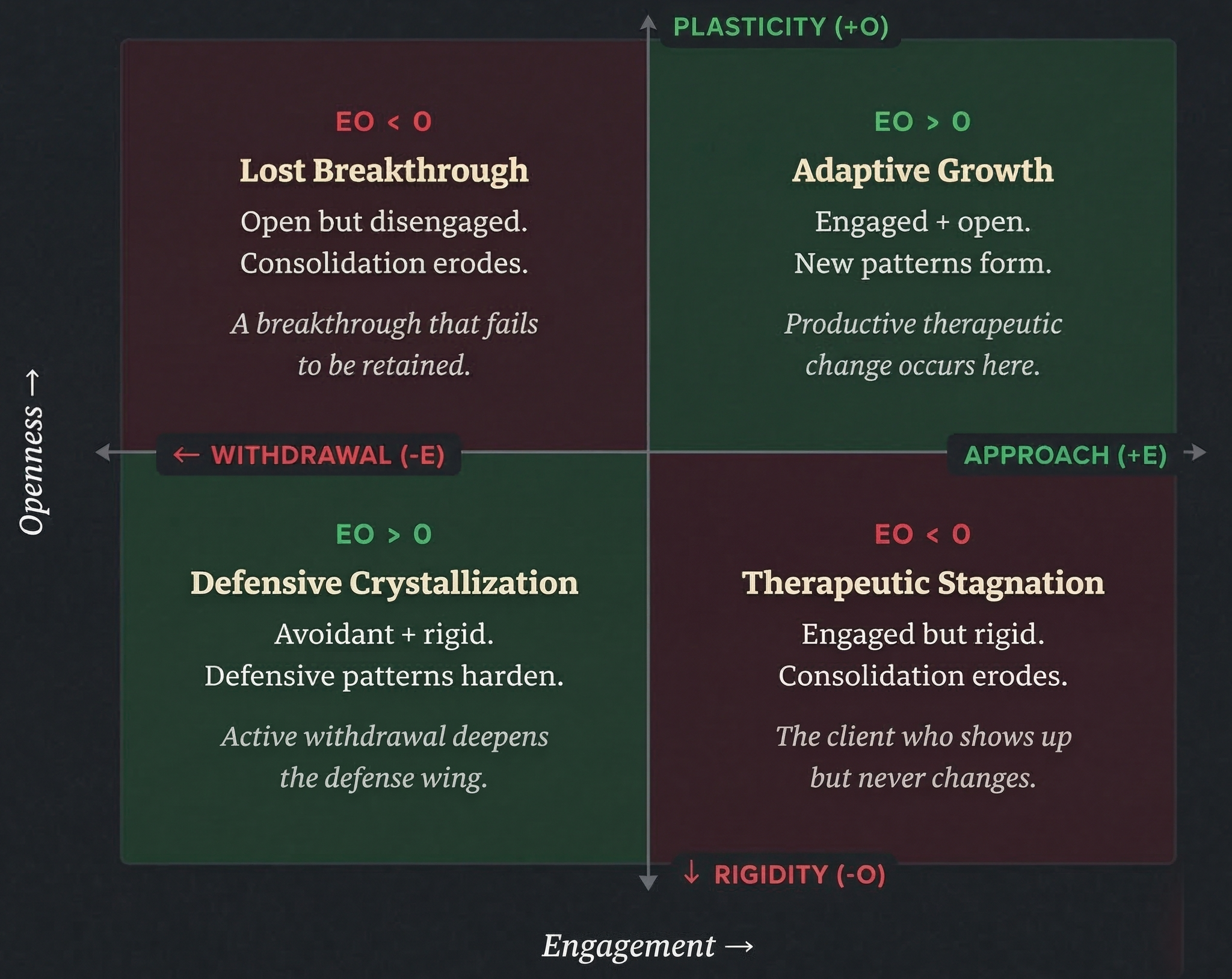
These four quadrants are model-generated predictions, not imposed categories. The mathematics dictates that only the positive-product quadrants (top-right and bottom-left) build consolidation. The negative-product quadrants (top-left and bottom-right) actively erode it. This is a direct consequence of the bilinear $EO$ term in Equation 3, and it is clinically plausible that engagement without flexibility, or flexibility without engagement, produces frustration and drift rather than durable change.
Each parameter has a specific interpretation. To manipulate them in real time and watch the attractor respond, see The Controls.
The parameter $\rho$ determines everything about the system's qualitative behavior. As it increases, the system passes through distinct dynamical regimes, each with a recognizable psychological signature.
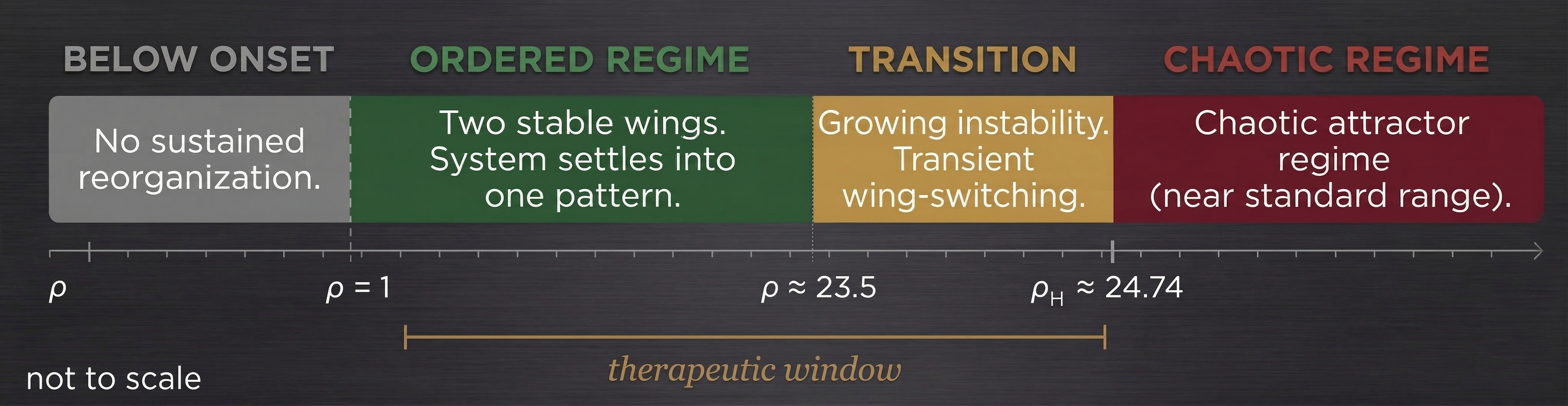
The Hopf bifurcation at $\rho_H \approx 24.74$ (for standard $\sigma = 10$, $\beta = 8/3$) is the main exact threshold in the standard Lorenz parameterization. It marks the point where the two nontrivial fixed points lose stability. But the approach to that threshold is not abrupt.
Classical analyses of the Lorenz system place the onset of sustained chaotic behavior below the Hopf point, near $\rho \approx 24.06$, with coexistence between a strange attractor and the two stable fixed points over part of the interval below $\rho_H$. In this site's implementation, visibly intermittent wing-switching begins around $\rho \approx 23.5$. That lower marker is best understood as an observed simulation/display threshold — the point at which long transient excursions become practically visible — rather than as a canonical bifurcation value.
In psychological terms, this transitional band corresponds to mounting oscillation between old and new patterns, longer periods of not knowing which way things will go, before the old equilibrium finally loses its hold. Once $\rho$ crosses the Hopf bifurcation, the fixed points are unstable and trajectories no longer settle there. In finite-time sweeps, the path back toward visibly ordered behavior can appear asymmetric because long transients and coexistence make destabilization and restabilization look different. That practical asymmetry is clinically suggestive, but its exact appearance depends on how the system is driven and observed.
This suggests a clinically significant prediction: there exists an optimal range of therapeutic intensity, bounded below by a subcritical threshold (below which little reorganization occurs) and above by an overwhelm threshold (above which the system fails to settle long enough to consolidate). The Intensity Cycle visualization shows what happens when $\rho$ rises through and falls back below these thresholds.
There is a second structural feature of the chaotic regime that matters as much as the bifurcation itself: sensitive dependence on initial conditions. In the chaotic regime, two trajectories that start from nearly identical points diverge exponentially over time, quantified by a positive largest Lyapunov exponent. The clinical implication is direct: even a perfect model of the coupling structure cannot predict which wing a specific individual will occupy after passing through a chaotic episode. The model predicts the landscape — which basins exist, where the main thresholds are, and what the regime structure looks like — but not the exact outcome for a given person. This is not a limitation of measurement or modeling alone. It is a structural property of deterministic chaos, and it places a principled bound on the predictability of therapeutic outcomes. The interactive visualization allows you to toggle a second trajectory and watch this divergence in real time.
The EOC model generates specific predictions that distinguish it from linear models and from vague formulations about therapeutic nonlinearity. Each prediction is testable with existing clinical instruments, though operationalizing them for formal study design would require further specification of measurement protocols and thresholds.
All trajectory computations on this site use fourth-order Runge-Kutta (RK4) integration with step size $dt = 0.005$ and downsampling for display. The Lyapunov exponent is computed via the standard renormalization method: a perturbation vector is evolved alongside the reference trajectory, periodically renormalized to unit length, and the running average of log-stretch rates converges to the largest Lyapunov exponent $\lambda_1$.
The bifurcation diagram is constructed by sweeping $\rho$ across its range, integrating for a transient period (discarded), then collecting local maxima of the consolidation variable $C$ over the remaining trajectory. The resulting structure is a familiar Lorenz bifurcation picture: stable fixed-point branches for lower $\rho$, loss of stability near $\rho_H$, and at larger $\rho$ a mix of chaotic bands and periodic windows. Near onset, the Lorenz transition is not well described as a simple low-$\rho$ period-doubling cascade.
A critical implementation note: at low $\rho$ values (below approximately 20–21 in this implementation), the trajectory can settle deeply into a wing basin and adiabatically track the fixed point with very little visually salient motion. The parameter $\rho_{\min}$ for any cycling visualization must therefore start above this range to produce visible dynamics within practical integration times.
The two nontrivial fixed points correspond to the growth wing ($+E^*, +O^*, C^*$) and the defense wing ($-E^*, -O^*, C^*$). Both share the same positive consolidation value $C^* = \rho - 1$. These fixed points exist for $\rho > 1$ and lose stability at $\rho_H = \sigma(\sigma + \beta + 3)/(\sigma - \beta - 1) \approx 24.74$ for the standard parameterization.
Equation 1 is an open hypothesis. The tracking relationship between engagement and openness is the least empirically grounded element. The psychotherapy literature supports the importance of both variables and their interaction, but the specific linear tracking ($dE/dt = \sigma(O - E)$) is a parsimony assumption. If future work shows that E and O can move independently for sustained periods, this equation would need modification, and exact Lorenz equivalence would be lost.
The three-variable reduction is undemonstrated. Existing empirical models use five or more state variables. The claim that these reduce to three near transitions is consistent with the slaving principle but has not been directly verified with clinical data. The reduction could fail if more than three slow modes remain active during transitions.
The model is deterministic. Real psychological dynamics include stochastic elements. A fuller treatment would incorporate Langevin-type noise terms, which Haken's framework supports but which are omitted here for clarity. The deterministic model captures the skeleton of the dynamics (the attractor topology, the bifurcation structure, the regime boundaries) but not the noise-driven fluctuations that would blur these boundaries in real data.
Observed threshold markers are partly implementation-dependent. Values such as $\rho \approx 23.5$ describe when instability becomes visibly salient under a particular integration scheme, observation window, and display method. They are useful practical markers for this site, but they should not be confused with universal Lorenz bifurcation constants.
Parameter estimation is not yet feasible. The model makes qualitative predictions about dynamical regimes and coupling relationships but does not yet support quantitative estimation of $\sigma$, $\rho$, or $\beta$ for individual patients. Bridging from qualitative prediction to individual parameter fitting would require high-frequency longitudinal data of a type that is becoming available (Schiepek et al., 2020) but is not yet standard.
The bilinear product $EO$ is an idealization. The bilinear product is the simplest polynomial encoding of the co-occurrence requirement. The underlying intuition is strongly supported empirically, but the functional form might be more complex. Saturating, threshold, or asymmetric interaction terms are all plausible alternatives. The EO product is the minimal form consistent with both the data and the Lorenz structure. Whether it is the correct form is an open question.
In the three-variable system above, ρ is a parameter. It is set from outside and held fixed. The two Explore pages treat it differently, and both go beyond the model documented on this page.
Externally Driven imposes a schedule on ρ, cycling it between roughly 19 and 31 with randomized timing and amplitude on each cycle. Pressure arrives on its own schedule and the system's task is to survive the crossing. The schedule is a modeling choice and nothing in the model derives it.
Internally Driven promotes ρ to a fourth state variable driven by the system's own activity:
where A measures the system's current turbulence, P is the rate at which pressure accumulates, γ is the rate at which activity discharges it, ε sets how slowly ρ moves relative to E, O and C, and η is optional additive noise. The claim is that quiescence accumulates pressure and upheaval discharges it, so the system generates its own crises without waiting for circumstance to deliver them.
This is a different dynamical system. The Lorenz identity established above holds for the E, O and C subsystem; adding the fourth equation produces a system with a Lorenz core and behavior the Lorenz system does not have, including a self-sustaining cycle and hysteresis. It is exploratory and is not part of the companion manuscript. The six predictions above belong to the three-variable model.
The equations above are not abstractions. They produce the trajectories you can watch, manipulate, and interrogate on the interactive pages. The strongest argument for the model is not the text. It is the behavior of the system when you change its parameters and recognize the patterns.